This section follows closely our publication in Ref. [Blin16a] .
See this publication for more detailed information and references.

Formalism

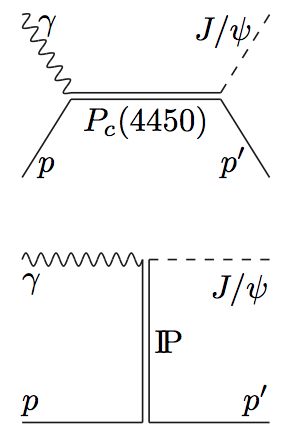
The two processes contributing to $\gamma\, p \to J/\psi p$ are shown in the figure. The top diagram represents the direct production of the $P_c(4450)$ resonance. The bottom diagram represent the background. The nonresonant background is expected to be dominated by the $t$-channel Pomeron exchange, and we saturate the $s$-channel by the $P_c(4450)$ resonance. In the following we consider only the most favored $J_r^P = 3/2^-$ and $5/2^+$ spin-parity assignments for the resonance. We adopt the usual normalization conventions, and express the differential cross section in terms of the helicity amplitudes $\bra{\lambda_{\psi}\lambda_{p^\prime}}T_r\ket{\lambda_\gamma \lambda_p}$, \begin{equation} \label{Edsigdcos} \frac{d\sigma}{d \cos\theta}= \frac{ 4\pi\alpha}{32 \pi s} \frac{p_f}{p_i} \frac{1}{4} \sum_{\lambda_\gamma,\lambda_p, \lambda_{\psi}, \lambda_{p'}} \left|\bra{\lambda_{\psi}\lambda_{p^\prime}} T \ket{\lambda_\gamma \lambda_p}\right|^2. \end{equation} Here, $p_i$ and $p_f$ are the incoming and outgoing center-of-mass frame momenta, respectively, $\theta$ is the center-of-mass scattering angle, and $W=\sqrt{s}$ is the total energy in the center-of-mass . Note that the electric charge $\sqrt{4\pi \alpha}$ is explicitly factored out from the matrix element. The contribution of the $P_c(4450)$ resonance is parametrized using the Breit-Wigner ansatz, \begin{align} \bra{\lambda_{\psi}\lambda_{p^\prime}}T_r\ket{\lambda_\gamma \lambda_p}= \frac {\bra{\lambda_{\psi}\lambda_{p^\prime}}T_{\text{dec}}\ket{\lambda_r}\bra{\lambda_r} T^\dagger_\text{em}\ket{\lambda_\gamma \lambda_p}} {M_r^2-W^2-\mathrm{i}\Gamma_rM_r}.\label{EBWamp} \end{align} The numerator is given by the product of photo-excitation and hadronic decay helicity amplitudes. The measured width is narrow enough to be approximated by a constant, $\Gamma_r=(39\pm 24)\mbox{ MeV}$. The angular momentum conservation restricts the sum over $\lambda_r$, the spin projection along the beam direction in the center of mass frame, to $\lambda_{r}=\lambda_{\gamma}-\lambda_{p}$. The hadronic helicity amplitude $T_\text{dec}$, which represents the decay of the resonance of spin $J$ to the $J/\psi$ state, is given by \begin{align} \bra{\lambda_{\psi}\lambda_{p'}}T_\text{dec}\ket{\lambda_r}= g_{\lambda_{\psi}\lambda_{p'}} d_{\lambda_r,\lambda_{\psi}-\lambda_{p'}}^{J}(\cos\theta), \end{align} where $g_{\lambda_{\psi}\lambda_{p'}}$ are the helicity couplings between the resonance and the final state. There are three independent couplings ($\lambda_{p^\prime} = \frac{1}{2}$, $\lambda_{\psi} = \pm 1,0$), the other three being related by parity. For simplicity, we assume all these couplings to be equal, i.e. $g_{\lambda_{\psi}\lambda'_p}\equiv g$. The helicity amplitudes and the partial decay width $\Gamma_{\psi p}$ are related by \begin{equation} \Gamma_{\psi p} = \mathcal{B}_{\psi p}\, \Gamma_r =\frac{\bar p_f}{32 \pi^2 M^2_{r}}\frac{1}{2J_{r}+1} \sum_{\lambda_{R}}\int d\Omega \,\vert\langle \lambda_{\psi}\lambda_{p'} \vert T_{dec} \vert \lambda_{R} \rangle |^2 = \frac{\bar p_f}{8\pi M_r^2} \frac{6g^2}{2J_r + 1} , \label{ampwidth} \end{equation} with $\mathcal{B}_{\psi p}$ being the branching ratio of $P_c \to J/\psi$ and $\bar p_f$ the momentum $p_f$ evaluated at the resonance peak. We assume that the $P_c(4450)$ decay is dominated by the lowest partial wave, with angular momentum $\ell=0$ for $J_r^P=3/2^-$ and $\ell=1$ for $J_r^P=5/2^+$. We recall that the following near-threshold behavior of the helicity amplitudes holds: $g \propto p_f^\ell$. The helicity matrix elements of $T_\text{em}$ are usually parametrized in terms of two independent coupling constants, $A_{1/2}$ and $A_{3/2}$, which are related to the matrix elements with $\lambda_r=1/2, 3/2$, respectively. The other two helicities $-1/2$ and $-3/2$ are constrained by parity. Using the standard normalization convention, in which the helicity couplings $A_{\lambda_{R}}$ have units of $\text{GeV}^{-1/2}$ and are proportional to the unit electromagnetic charge, \begin{equation} \label{a12a32sec} \langle \lambda_{\gamma}\lambda_{p} \left| T_\text{em} \right| \lambda_{R} \rangle =\frac{W}{M_{r}}\sqrt{\frac{8M_{N}M_{r} \bar p_{i}}{4\pi\alpha}} \sqrt{\frac{\bar p_i}{p_i}}A_{\lambda_{R}}, \end{equation} with $\bar{p}_i$ the momentum $p_i$ evaluated at the resonance peak. The electromagnetic decay width $\Gamma_\gamma$ is given by \begin{equation} \label{a12a32width1} \Gamma_{\gamma}= \frac{\bar p_i^2} {\pi}\frac{2M_{N}}{(2J_{r}+1)M_{r}} \left[ \left | A_{1/2} \right |^{2}+\left | A_{3/2} \right|^{2} \right]. \end{equation}

Model

The photon helicity amplitudes for a pentaquark are not known. To rely on data as much as possible, we start by following Ref. [Kar16a] and assume a vector-meson dominance (VMD) relation for the transverse vector-meson helicity amplitudes \begin{equation} \bra{\lambda_{\gamma}\lambda_p}T_\text{em} \ket{\lambda_r} = \frac{\sqrt{4\pi \alpha} f_\psi}{M_\psi} \bra{\lambda_{\psi}=\lambda_\gamma ,\lambda_p}T_\text{dec} \ket{\lambda_r}, \label{vmd} \end{equation} with $f_\psi$ being the $J/\psi$ decay constant which is proportional to the electromagnetic current matrix elements, $\bra{0} J^\mu_\text{em} (0)\ket{J/\psi( p,\lambda)} = \sqrt{4\pi \alpha} f_\psi M_\psi \epsilon^\mu(p,\lambda).$ The decay constant is related to the $J/\psi$ wave function via the Van~Royen-Weisskopf relation, and can be estimated from the leptonic decay width of the $J/\psi \to l^+l^-$, yielding $f_\psi=280$ MeV. Finally, the VMD hypothesis leads to \begin{align} \Gamma_\gamma=4\pi \alpha \,\Gamma_{\psi p} \left(\frac{f_{\psi}}{M_{\psi}}\right)^2 \left(\frac{\bar p_i}{\bar p_f}\right)^{2\ell + 1} \times \frac{4}{6}, \label{eqvecdom} \end{align} with the factor $4/6$ due to the fact that in Eq. \eqref{vmd} only the transverse polarizations of the $J/\psi$ contribute. Again, we use $\ell=0$ for $J_r^P=3/2^-$ and $\ell=1$ for $J_r^P=5/2^+$. With the help of Eqs. \eqref{a12a32width1} and \eqref{eqvecdom}, one can constrain the size of the photocouplings. The background in the resonance region is assumed to be dominated by diffractive production, which we parametrize by an effective, helicity-conserving, Pomeron exchange model: \begin{align} \langle \lambda_\psi\lambda_{p^\prime}|T_{P} |\lambda_\gamma \lambda_p\rangle = iA~\left(\frac{s-s_t}{s_0}\right)^{\alpha(t)}~e^{b_0 t'} \delta_{\lambda_p\lambda_{p'}}\delta_{\lambda_{\psi}\lambda_\gamma}. \label{EqPom} \end{align} Here $s_0=1\mbox{ GeV}^2$ is fixed and $t' = t-t_\text{min}$. The Pomeron trajectory is given by $\alpha(t)=\alpha_0 + \alpha' \: t $, where $\alpha_0$ and $\alpha'$ are parameters to be determined, as well as the normalization $A$, the effective threshold parameter $s_t$, and the $t$-slope parameter $b_0$.

There seems to be a rapid decrease of the cross section in the threshold region and the shift parameter $s_t$ is introduced to enable a smooth connection between the high energy, $W \sim 100\mbox{ GeV}$, and the threshold.

The result is presented below for the model of Table I in Ref. [Blin16a] .
From left to right, the plots are:

• The differential cross section in the forward direction as a function of the photon energy $\frac{d\sigma}{dE_\gamma}(t' = 0)$.
• The total cross section as a function of the photon energy $\sigma_\text{tot}(E_\gamma)$.
• The angular distribution at the peak $\frac{d\sigma}{dt}(s = M_r^2)$.

References

[Blin16a]
A. N. Hiller Blin et al. (JPAC collaboration),
``Studying the $P_c$(4450) resonance in $J/\psi$ photoproduction off protons,'' Phys. Rev. D 94, 034002 (2016),

[Kar16a]
M. Karliner and J. L. Rosner,
``Photoproduction of Exotic Baryon Resonances,'' Phys. Lett. B752, 329 (2016).

Resources

• Publication: [Blin16a]
• Material:
  • Web.tar.gz, compressed file with the codes. See below for the description of the files,
  • C++ codes in a zip file,
  • Formalism in a zip file
• Contact person: Astrid H. Blin
• Last update: December 2017

Description of the files in the compressed archive Web.tar.gz:

Simulation

We invite the users to reproduce our plots with their own set of parameters.
In order to do so, the possible choices are for:

• The fitting parameteres of the paper $\alpha_0$, $\alpha'$, $A$, $s_t$, $b_0$ and $\mathcal{B}_{\psi p}$;
  Choose $\mathcal{B}_{\psi p}=0$ in order to reproduce only the Pomeron background;
• The physical mass and width of the $P_c(4450)$, $M_r$ and $\Gamma_r$, to enable varying them within their errors;
• The spin assignment $3/2$ or $5/2$;
• The size of the smearing due to the experimental resolution;
• The photocoupling assignment: $r_{1/2} = A_{1/2}/(|A_{1/2}|^2+|A_{3/2}|^2)^{1/2}$. The norm $|A_{1/2}|^2+|A_{3/2}|^2$ is fixed.
  
• Finally, the observable to plot:
  • The differential cross section in the forward direction as a function of the photon energy,
  • The total cross section as a function of the photon energy,
  • The angular behaviour of the differential cross section at the resonance peak,
  • The asymmetry $K_{LL}$ in the forward direction as a function of the photon energy,
  • The angular behaviour of the asymmetry $K_{LL}$ at the resonance peak,
  • The spin-density matrix element (SDME) $\rho_{00}$ in the forward direction as a function of the photon energ
  • The angular behaviour of the SDME $\rho_{00}$ at the resonance peak,
  • The SDME $\rho_{10}$ in the forward direction as a function of the photon energy,
  • The angular behaviour of the SDME $\rho_{10}$ at the resonance peak,
  • The SDME $\rho_{1-1}$ in the forward direction as a function of the photon energy,
  • The angular behaviour of the SDME $\rho_{1-1}$ at the resonance peak.
• If you choose the differential cross section or any of the SDMEs in the forward direction,
  you can choose the maximal energy to display, $E_\text{max}$.