This page concerns the amplitudes for pion-nucleon scatterings. For the Finite Energy Sum Rules pages, go to the FESR $\pi N$ page

We present the model published in [Mat15b] concerning pion-nucleon scatterings.
We use the CGLN invariant amplitudes $A$ and $B$ defined in [Chew57b].
The SAID solution is used at low energy. At higher energy, a Regge parametrization is used.
The parameters of the Regge parametrization are determined by fitting the high energy data.
The fitting procedure is detailed in [Mat15b] . We report here only the main features of the model.
The code can be downloaded in Resources section and simulated in the Simulation section.

Formalism

The pion-nucleon scattering is a function of 2 variables. The first is the beam momentum in the laboratory frame $p_\text{lab}$ (in GeV) or the total energy squared $s=W^2$ (in GeV$^2$). The second is the cosine of the scattering angle in the rest frame $\cos\theta$ or the momentum transfered squared $t$ (in GeV$^2$).
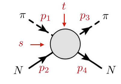
The momenta of the particles are:
$p_1$ and $p_3$ (incoming and outgoing pions), $p_2$ (target) and $p_4$ (recoil).
The helicities of the proton are $\lambda_2$ and $\lambda_4$.
The pion mass is $\mu$ and the proton mass is $M$.
The Mandelstam variables, $s=(p_1+p_2)^2$, $t=(p_1-p_3)^2$, $u=(p_1-p_4)^2$ are related through $s+t+u=2M^2+2\mu^2$.

Since the $s-$channel, $\pi N \to \pi N$, and the $u-$channel, $\pi \bar N \to \pi \bar N$, are related by conjugation charge and isospin symmetry, the dispersion relations can be recast in a symmetric form by using the crossing variable $\nu$ defined by \begin{align} \nu = \frac{s-u}{4M} = E_\text{lab} + \frac{t}{4M}. \end{align}

The scattering amplitude $\left(T_{\lambda_2 \lambda_4} \right)_{ji}^{ba}$ for the reaction $\pi^a N_i \to \pi^b N_j$ is decomposed into scalar amplitudes: \begin{align} \left(T_{\lambda_2\lambda_4}\right)_{ji}^{ba} = \bar u(p_4,\lambda_4) \left[ A_{ji}^{ba} + \frac{1}{2} (p_1\!\!\!\!\! /\ +p_3\!\!\!\!\! / \ ) B_{ji}^{ba} \right] u(\lambda_2,p_2). \label{eq:T} \end{align} The indices $(a,b)$ and $(i,j)$ are isospin indices for $I=1$ (pion) and $I=\frac{1}{2}$ (nucleon).
It is often convenient to define another scalar amplitudes denoted by $C$ or $A'$ \begin{align} C \equiv A' \equiv A + \frac{M(s-u)}{4M^2-t} B = A + \frac{\nu}{1-t/4M^2} B. \end{align} In the isospin limit, the scalar amplitudes admit an isospin decomposition. For the label, one can choose the $s-$channel isospin indices $\left(\frac{1}{2}\right)$ and $\left(\frac{3}{2}\right)$ or the $t-$channel isospin indices $\left( + \right)$ and $\left( - \right)$. They are related by \begin{align} A^{(\frac{1}{2})} &= A^{(+)} + 2A^{(-)}, & A^{(\frac{3}{2})} &= A^{(+)} - A^{(-)}. \end{align} The relation between physical reactions are isospin amplitudes $F = A,B,C$ are \begin{align} \pi^\pm p &\to \pi^\pm p & F^{(+)} \mp F^{(-)} \\ \pi^\pm n &\to \pi^\pm n & F^{(+)} \pm F^{(-)} \\ \pi^- p &\to \pi^0 n & -\sqrt{2} F^{(-)} \end{align}

For given isospin combination (isospin indices are omitted for simplicity), the scattering amplitudes \eqref{eq:T} are written as \begin{align} \nonumber T_{++} &= 8\pi W \left(\frac{1+z}{2}\right)^{\frac{1}{2}} \left(f_1+f_2\right),\\ T_{+-} &= 8\pi W \left(\frac{1-z}{2}\right)^{\frac{1}{2}} \left(f_1-f_2\right), \label{eq:ampl} \end{align} The short-hand notation for the nucleon helicities is $\pm\equiv \pm \frac{1}{2}$.
$z = \cos\theta = 1 + t/2q^2$ is the cosine of the scattering angle with $q$ the break-up momentum between the pion and the nucleon.
The partial waves decomposition of the reduced helicity amplitudes $(f_1,f_2)$ read \begin{align} \nonumber f_1(s,t) &= \frac{1}{q}\sum_{\ell=0}^\infty f_{\ell+}(s) P_{\ell+1}^\prime(z) - \frac{1}{q}\sum_{\ell=2}^\infty f_{\ell-}(s) P_{\ell-1}^\prime(z)\\ f_2(s,t) &= \frac{1}{q}\sum_{\ell=1}^\infty\left[ f_{\ell-}(s) - f_{\ell+}(s)\right] P_{\ell}^\prime(z) \label{eq:f} \end{align} $f_{\ell\pm}$ are the partial wave amplitudes with parity $(-1)^{\ell+1}$ and total angular momentum $J=\ell\pm1/2$.
Fiinally the relations between the reduced helicity amplitudes and the scalar amplitudes are \begin{align} \nonumber \frac{1}{4\pi} A & = \frac{W+M}{E+M} f_1 - \frac{W-M}{E-M} f_2, \\ \frac{1}{4\pi} B & = \frac{1}{E+M} f_1 + \frac{1}{E-M} f_2. \label{eq:AB} \end{align} $E = (s + M^2 − \mu^2)/2W)$ is the nucleon energy.

In these conventions, the observables are:

• Total cross section \begin{align} \nonumber \sigma_{\text{tot}}&= \frac{1}{2 qW}\ [T_{++} + T_{+-}]|_{t=0} = \frac{1}{p_\text{lab}} \text{Im} A'(s,t=0) \end{align}
• Differential cross section \begin{align}\nonumber \frac{d\sigma}{dt}&= \frac{\pi}{q^2} \left(\frac{1}{8\pi W}\right)^2\left(|T_{++}|^2 + |T_{+-}|^2\right) \\ \nonumber &= \frac{1}{\pi s} \left(\frac{M}{4q}\right)^2 \bigg[ \left(1- \frac{t}{4M^2}\right) |A'|^2 - \frac{t}{4M^2} \left(\frac{st/4M^2 + p^2_\text{lab} }{1-t/4M^2} \right) |B|^2\bigg] \end{align} Please note the missprint in Eq. (10b) in the publication [Mat15b] .
• Polarization observable \begin{align}\nonumber P &= \frac{2\,\text{Im} \ T_{++}T^{*}_{+-}}{|T_{++}|^2 + |T_{+-}|^2} = -\frac{\sin\theta}{16\pi W} \frac{\text{Im}\left(A' B^*\right)}{d\sigma/dt}, \end{align}

Model

At low energy only a finite number of partial waves contribue to the scattering amplitudes.
We use the SAID WI08 solution, published in [Wor12a] , valid up to $p_\text{lab}=2.5$ GeV.
The SAID solution, extracted from the SAID webpage , is provided by 8 waves for both parity and both $s-$channel isospin: \begin{align*} && P11 && D13 && F15 && G17 && H19 \qquad I111 \qquad J113 \\ S11 && P13 && D15 && F17 && G19 && H111\qquad I113 \qquad J115 \\ && P31 && D33 && F35 && G37 && H39 \qquad I311 \qquad J313 \\ S31 && P33 && D35 && F37 && G39 && H311 \qquad I313 \qquad J315 \end{align*} In the spectroscopic notation, $L (2I) (2J)$.
Recall that the amplitudes $f_{1,2}$ and $f_{\ell\pm}$ have isospin indices, omitted in \eqref{eq:ampl}, \eqref{eq:f} and \eqref{eq:AB}.

At high energy $p_\text{lab}>2.5$ GeV, we use a Regge parametrization for the invariant amplitudes.
The $t-$channel isospin-1 amplitudes involve a $\rho$ Regge pole: \begin{align} \nonumber A'^{(-)} &= \pi C^\rho_0\frac{\left[(1+C^\rho_2)e^{C^\rho_1 t}-C^\rho_2\right]}{\Gamma(\alpha_\rho+1)} \frac{e^{-i\pi \alpha_\rho}-1}{2 \sin\pi\alpha_\rho} \nu^{\alpha_\rho}, \\ \nonumber \nu B^{(-)} &= -D^\rho_0 e^{D^\rho_1 t} \frac{\pi}{\Gamma(\alpha_\rho)} \frac{e^{-i\pi \alpha_\rho}-1}{2 \sin\pi\alpha_\rho} \nu^{\alpha_\rho}. \end{align}

The $t-$channel isospin-0 amplitudes involve the Pomeron pole and a $f$ Regge pole: \begin{align} \nonumber A'^{(+)} & = A'^{\mathbb P} + A'^f & B^{(+)} & = B^{\mathbb P} + B^f \end{align} The Regge parametrization for these poles are given by \begin{align} \nonumber A'^{\mathbb P} &= -C_0^{\mathbb P}e^{C_1^{\mathbb P} t}\frac{\pi}{\Gamma(\alpha_{\mathbb P})} \frac{e^{-i\pi \alpha_{\mathbb P}}+1}{2 \sin\pi\alpha_{\mathbb P}} \nu^{\alpha_{\mathbb P}}, & \nu B^{\mathbb P} &= A'^{\mathbb P},\\ \nonumber A'^f &= -C_0^fe^{C_1^f t}\frac{\pi}{\Gamma(\alpha_f)} \frac{e^{-i\pi \alpha_f}+1}{2 \sin\pi\alpha_f} \nu^{\alpha_f}, & \nu B^f &= A'^f. \end{align} In the Regge parametrization, the crossing variable $\nu$ is expressed in GeV.
The trajectories and the other parameters are given in the Table I of [Mat15b] .

The amplitudes available below are constructed as follow:
The SAID solution is used at low energies $\nu < 1.5$ GeV,
the Regge model is used at high energies, $\nu > 2.1$ GeV,
and between these thresolds we use a linear interpolation between SAID and the Regge parametrization.

The range of validity of the Regge parametrization is $t\in [-1,0]$ GeV$^2$.
However the formula are analytic in $t$ and can be extended for $t< -1$ GeV$^2$.
The Regge model does not include backward baryonic exchanges.
Hence the model underestimates the backward region.

As an example, we display the total cross sections $\sigma(\pi^\pm p \to X)$:

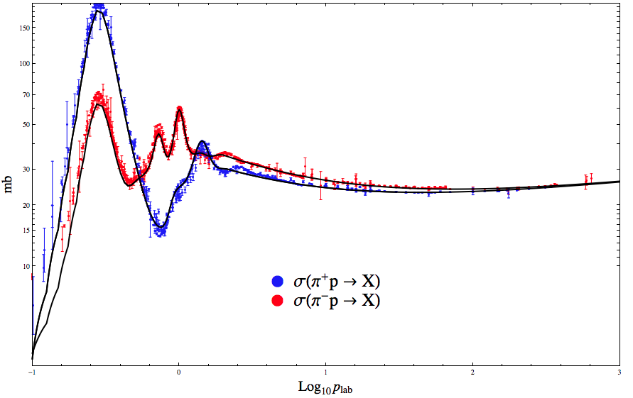
The data are taken from the Review of Particle Physics

References

[Chew57b]
G.F. Chew, M.L. Goldberger, F.E. Low and Y. Nambu,
``Application of Dispersion Relations to Low-Energy Meson-Nucleon Scattering,'', Phys. Rev. 106, (1957) 1337.

[Wor12a]
R.L. Workman, R.A. Arndt, W.J. Briscoe, M.W. Paris, I.I. Strakovsky
``Parameterization dependence of T matrix poles and eigenphases from a fit to $\pi N$ elastic scattering data,''
arXiv:1204.2277 [hep-ph], Phys. Rev. C 86, 035202 (2012)

[Mat15b]
V. Mathieu, I. V. Danilkin, C. Fernandez-Ramirez, M. R. Pennington, D. Schott, A. P. Szczepaniak and G. Fox
``Toward Complete Pion Nucleon Amplitudes,'' arXiv:1506.01764 [hep-ph], Phys. Rev. D 92, 074004 (2015)

Resources

• Publications: [Mat15a] and [Wor12a]
• SAID partial waves: compressed zip file
• C/C++: MainPiN.c
• Fortran: PiN.f, cgamma.f90
• Input file: param.txt, list.txt
• Output files: output0.txt, output1.txt, SigTot.txt , Observables0.txt, Observables1.txt, Observables2.txt.
• Contact person: Vincent Mathieu
• Last update: December 2016

Simulation