

 This page concerns the Finite Energy Sum Rules for pion photoproduction
from the publication [Mat18b] .
A brief description of the formalism is given in the Formalisms section.
Please see the publication [Mat18b] for further details.
Both side of the sum rules are compared interactively in the Simulation section.
The user can also display the observables at high energies.
The codes can be downloaded in Resources section.
Formalism
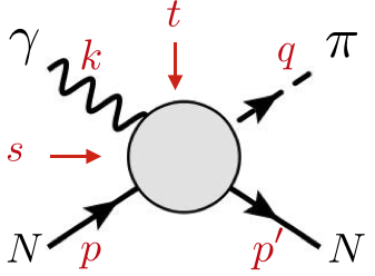
The photoproduction of a single pion is a function of 2 variables.
We are using the the momentum transfered squared $t$ and
the crossing variable $\nu$ defined by
\begin{align}
\nu = \frac{s-u}{4M} = E_\gamma^\text{lab} + \frac{t-\mu^2}{4M}.
\end{align}
The pion mass is $\mu$ and the proton mass is $M$.
The Mandelstam variables, $s = (k+p)^2$, $t = (k-q)^2$ and $u= (k-p')^2$, satisfy $s+t+u= 2M^2+\mu^2$.
The scattering amplitude $\left(A _{ji}^{a}\right) _{\lambda', \lambda \lambda_\gamma}$
for the reaction $\gamma (k, \lambda_\gamma) N_i (p, \lambda) \to \pi^a (q) N_j (p',\lambda')$
is decomposed into the CGLN scalar amplitudes .
Assuming isospin symmetry, we can attach to each scalar amplitude an isospin index:
\begin{align}
\left(A _{ji}^{a}\right) _{\lambda', \lambda \lambda_\gamma} & =
\sum_{k = 1}^4 \bar u(p',\lambda')\ (A_{ji}^{a})_k(s,t) M_k(s,t,\lambda_\gamma)\ u(p, \lambda). \label{eq:T} \\
(A_{ji}^{a})_k & = (\tau)_{ji}^{a} A_k^{(0)} + \delta_{ji}\delta^{a3} A_k^{(+)}
+ \frac{1}{2}\left[\tau^{a},\tau^{3} \right]_{ji} A_k^{(-)}
\end{align}
The indices $a$ and $(i,j)$ are isospin indices for $I=1$ (pion) and $I=\frac{1}{2}$ (nucleon).
The $\tau$ matrices are the Pauli matrices and
the structures $M_k(s,t,\lambda_\gamma)$ are defined in [Mat15a] .
The scalar functions have good isospin and $G$-parity in the $t$-channel.
Their properties are summarized in the following table:
| $A_k^{(\sigma)}$ | | | $I^G$ | $P(-1)^J$ | $\tau$ | $J^{PC}$ | | | lightest meson | |
| $--$ | | | $--$ | $----$ | $--$ | $-----$ | | | $------$ | |
| $A_{1,4}^{(0)}$ | | | $1^+$ | $+1$ | $-1$ | $(1,3,\ldots)^{--}$ | | | $\rho(770)$ | |
| $A_{1,4}^{(+)}$ | | | $0^-$ | $+1$ | $-1$ | $(1,3,\ldots)^{--}$ | | | $\omega(782)$ | |
| $A_{1,4}^{(-)}$ | | | $1^-$ | $+1$ | $+1$ | $(2,4,\ldots)^{++}$ | | | $a_2(1320)$ | |
| $--$ | | | $--$ | $----$ | $--$ | $-----$ | | | $------$ | |
| $A_{2}^{(0)}$ | | | $1^+$ | $-1$ | $-1$ | $(1,3,\ldots)^{+-}$ | | | $b_1(1235)$ | |
| $A_{2}^{(+)}$ | | | $0^-$ | $-1$ | $-1$ | $(1,3,\ldots)^{+-}$ | | | $h(1170)$ | |
| $A_{2}^{(-)}$ | | | $1^-$ | $-1$ | $+1$ | $(2,4,\ldots)^{-+}$ | | | $\pi(140)$ | |
| $--$ | | | $--$ | $----$ | $--$ | $-----$ | | | $------$ | |
| $A_{3}^{(0)}$ | | | $1^+$ | $-1$ | $+1$ | $(1,3,\ldots)^{+-}$ | | | $\rho_2(-)$ | |
| $A_{3}^{(+)}$ | | | $0^-$ | $-1$ | $+1$ | $(1,3,\ldots)^{+-}$ | | | $\omega_2(-)$ | |
| $A_{3}^{(-)}$ | | | $1^-$ | $-1$ | $-1$ | $(2,4,\ldots)^{-+}$ | | | $a_1(1260)$ | |
| $--$ | | | $--$ | $----$ | $--$ | $-----$ | | | $------$ |
The signature of the exchange, $\tau = (-1)^J$, provides the crossing properties of the scalar function,
i.e. $A_k^{(\sigma)}(-\nu-i\epsilon, t) = \tau A_k^{(\sigma)}(\nu+i\epsilon, t)$.
The relation to scalar function for given reaction is
\begin{align*}
A\left(\gamma p \to \pi^0 p \right)&= A^{(+)} + A^{(0)}, &
A\left( \gamma p \to \pi^+ n \right)&= \sqrt{2} \left(A^{(0)} +A^{(-)} \right), \\
A\left(\gamma n \to \pi^0 n \right)&= A^{(+)} - A^{(0)} &
A\left(\gamma n \to \pi^- p\right)&= \sqrt{2} \left(A^{(0)} -A^{(-)} \right),\\
\end{align*}
If, for an amplitude $A_i^{(\sigma)}$, we assume a sum of Regge poles of the form:
\begin{align}
\text{Im } R_{i}^{(\sigma)}(\nu,t) = \sum_{j} \beta^{(\sigma)}_{ij}(t) (r \nu)^{\alpha_j(t)-1}.
\end{align}
The scale factor is chosen to be $r = 1$ GeV$^{-1}$.
The finite energy sum rules are
\begin{align}
B_k^{(\sigma)}\frac{\pi}{\Lambda} \left(\frac{\nu_N}{\Lambda}\right)^k
+ \int_{\nu_0}^{\Lambda} \text{Im } A_i^{(\sigma)}(\nu,t) \left(\frac{\nu}{\Lambda}\right)^k \frac{d \nu}{\Lambda} =
\sum_j \beta^{(\sigma)}_{ij}(t) \frac{(r \Lambda)^{\alpha_j(t)-1}}{\alpha_j(t)+k} \label{eq:FESR}
\end{align}
The moment $k$ is even (odd) for an even (odd) amplitudes, i.e. $\tau (-1)^k = +1$
The Born term are given in the table:
| $(\sigma)$ | | | $(0)$ | $(+)$ | $(-)$ | | | values |
| $--$ | | | $----$ | $----$ | $----$ | | | $------$ |
| $B_1^{(\sigma)}$ | | | $-\frac{1}{2}\frac{eg}{2 M}$ | $-\frac{1}{2}\frac{eg}{2 M}$ | $-\frac{1}{2}\frac{eg}{2 M}$ | | | $e = 0.303$ |
| $B_2^{(\sigma)}$ | | | $\frac{1}{t-\mu^2}\frac{eg}{2 M}$ | $\frac{1}{t-\mu^2}\frac{eg}{2 M}$ | $\frac{1}{t-\mu^2}\frac{eg}{2 M}$ | | | $g = 13.54$ |
| $B_3^{(\sigma)}$ | | | $\frac{\kappa_p+\kappa_n}{4 M}\frac{eg}{2 M}$ | $\frac{\kappa_p-\kappa_n}{4 M}\frac{eg}{2 M}$ | $\frac{\kappa_p-\kappa_n}{4 M}\frac{eg}{2 M}$ | | | $\kappa_p = 1.78$ |
| $B_4^{(\sigma)}$ | | | $\frac{\kappa_p+\kappa_n}{4 M}\frac{eg}{2 M}$ | $\frac{\kappa_p-\kappa_n}{4 M}\frac{eg}{2 M}$ | $\frac{\kappa_p-\kappa_n}{4 M}\frac{eg}{2 M}$ | | | $\kappa_n = -1.91$ |
| $--$ | | | $----$ | $----$ | $----$ | | | $------$ |
Model
At high energy $E_\gamma^\text{lab}>3.0$ GeV, we use a Regge parametrization for the invariant amplitudes.
The residue of the Regge pole $j$ in the amplitude $i$ is of the form (omitting the indices)
\begin{align}
\beta(t) & = \left[\alpha(t)\right]^\kappa\ t^\delta
\times \beta e^{b t} (1-\gamma_1 t) (1-\gamma_2 t)
\end{align}
We use linear trajectories $\alpha(t) = \alpha(0) + \alpha' t $.
The left-hand side (LHS) of the sum rules can be computed from any low energy model given in term of multipoles.
Below the user could generate the LHS of the FESR with the models:
SAID,
MAID
Other models will be included soon. Contact
Vincent Mathieu (mathieuv.at.indiana.edu)
if you want your models to be included here.
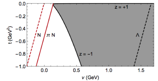 The integration in the FESR Eq. \eqref{eq:FESR} is performed at fixed $t$.
For $t\neq t_{\text{min}}$, the integral involve an unphysical region.
The physical region ($|z = \cos\theta| \le 1$) is the grey area in the figure.
The solid (dashed) red line represent the $\pi N$ threshold (nucleon pole).
The extrapolation outside the physical region is performed by
evaluating the Legendre polynomials for $\cos\theta \le -1$.
High partial wave might compromise the numerical stability of the amplitudes in the unphysical region.
For this reason, we limit the number of waves to $L_\text{max} = 5$ for the models in the resonance region.
References
[Mat18b]
V. Mathieu, J. Nys, C. Fernandez-Ramirez, A. N. Hiller Blin, A. Jackura,
A. Pilloni, A. P. Szczepaniak and G. Fox
``Structure of Pion Photoproduction Amplitudes,''
arXiv:1806.08414 [hep-ph],
Phys. Rev. D 98, 014041 (2018)
[Mat15a]
V. Mathieu, G. Fox and A. P. Szczepaniak
``Neutral Pion Photoproduction in a Regge Model,''
arXiv:1505.02321 [hep-ph],
Phys. Rev. D 92, 074013 (2015)
Resources
- Publications: [Mat18b]
- Multipoles: SAID, MAID
- C/C++: FESR-PiPhot-Low.c, FESR-PiPhot-Regge.c
- Input file: multipoles-model.txt, Simulation-param.txt, Trajectories.txt, Residues.txt.
- Contact person: Vincent Mathieu (mathieuv.at.indiana.edu)
- Last update: June 2018
- FESR-PiPhot-Low.c:
- Read_Multipoles reads the multipoles from files.
- Smooth_Multipoles interpolates between the multipoles at fixed $s$.
- MltPole2F returns the CGLN $F_i$ from multipoles.
- CGLNA2F converts CGLN $A_i$ into CGLN $F_i$ at fixed $t$ and $s$.
- CGLNF2A converts CGLN $F_i$ into CGLN $A_i$ at fixed $t$ and $s$.
- amplHi converts CGLN $F_i$ into $H_i$ amplitudes at fixed $t$ and $s$.
- kinematics computes all relevant kinemtical quantities at fixed $t$ and $s$ and store them into a structure.
- FESR-PiPhot-Regge.c:
- FESR_Regge returns the FESR at fixed $t$.
- Ai_Regge returns the scalar amplitudes at fixed $t$ and $s$.
- DSig_Regge returns the differential cross section at fixed $t$ and $s$.
- Pol_Regge returns the polarization observables at fixed $t$ and $s$.
- Simulation-param.txt
Elab tmin tmax dt cutoff k1 k2 wmin wmax dw t0
- Elab: Lab energy for printing the observables for high energy
- tmin tmax dt: interval in t for the FESR
- wmin wmax dw: interval in $W=\sqrt{s}$ for printing Ai
- t0: print Ai at t = t0
- cutoff: W-max for the FESR
- k1 k2: moments of the FESR
- Trajectories.txt
Intercept and slopes of 10 trajectories. Only the 8 first are used in this model. - Residues.txt
Parameters of the 12x2 residues $\beta(t)$.
Each amplitudes contains 2 contribution, the leading Regge pole and a sub-leading contribution.
In this model, the unnatural amplitude has only one contribution. The parameters of their sub-leading pole are set to zero.
Each line is $j$, $\kappa$, $\delta$, $\beta_0$, $b$, $\gamma_1$, $\gamma_2$.
Simulation
The code compute both side of the FESR Eq. \eqref{eq:FESR} with the moment $k_1$ (odd amplitudes) and $k_2$ (even amplitudes).The user can choose the moments $k_{1,2}$. They must be even positive integers.
$k_1$ must be odd and $k_2$ must be even.
The suggested cutoff is $W_\text{max}$ is 2 GeV. The SAID model can be used up to 2.4 GeV and MAID up to 2.0 GeV
Note that imposing a cutoff above the range of validity of a solution might lead to misleading results.
The limit of validity of the models can be read from the partial waves files.
One can print the observables (differential cross section and $\Sigma,T,R$ asymmetries) using the Regge model.
The default value to compute the observables is $E^\text{lab}_\gamma = 9$ GeV.
The default $t$ range for the observables and the FESR is $t\in [-1,0]$ GeV$^2$.
The kinematical quentities are expressed in GeV.
The parameters (trajectories and residues) of the model can be changed. The defaults values are taken from [Mat18b] .