Introduction

Hadronic finite state interactions for $\eta\rightarrow 3\pi$ decay is essential in order to reproduce the data and understand known discrepancies between Dalitz plot parameters from experiment and chiral perturbation theory. Our results are based on the Khuri-Triman equations which were solved by the Pasquier inversion technique. The subtraction constants are used as free fitting paramters. On this site, we briefly present the formalism of our approach, and provide a example of descriptions of three-body effect based on WASA-at-COSY Dalitz distribution [WASAatCOSY:2014]. The C++ code and its instruction is also provided in the end.

Formalism

The amplitudes that describe $\eta\rightarrow3\pi$ charge and neutral decay are given by, \begin{align} & A^{C}(s,t,u) = \sum_{L=0}^{L_{max}}\frac{(2L+1)}{2} \bigg [ \frac{2}{3}\,P_{L}(z_{s}) \left ( \, a_{0 L} (s ) - a_{2 L} (s) \right) \nonumber \\ & \quad \quad \quad \quad \quad \quad \quad \quad \quad \quad \quad \quad + P_{L}(z_{t}) \left ( \,a_{1 L} (t) + a_{2 L} (t) \right)-P_{L}(z_{u}) \left ( \,a_{1 L} (u) - a_{2 L} (u) \right) \bigg ]\,, \\ & A^{N}(s,t,u)=\sum_{L=0}^{L_{max}}\frac{(2L+1)}{3} \bigg[ \,P_{L}(z_{s})\left(\,a_{0 L} (s) +2a_{2 L} (s) \right) + (s \to t) + (s\to u) \bigg]\,. \label{ampn} \end{align} where $A^{C/N}(s,t,u)$ are the charge/neutral decay amplitudes of the three Mandelstam variables satisfying $s+t+u = M^2 + m_{1}^2+m_{2}^{2}+m_{3}^{2}$. $P_{L}(z_s)$ is the Legendre polynomial and $z_s$ is a cosine of the center-of-mass scattering angle $\theta_s$, \begin{equation} z_s \equiv\cos\theta_s=\frac{s\,(t-u)+ (m_{1}^{2}-m_{2}^{2})\,(M^{2} -m_{3}^{2})}{ \lambda^{1/2}(s,M^{2} ,m_{3}^2)\,\lambda^{1/2}(s,m_{1}^2,m_{2}^2) }\, = \frac{s\,(t-u)+ (m_{1}^{2}-m_{2}^{2})\,(M^{2} -m_{3}^{2})}{ K(s) }\,.\label{zs} \end{equation} The usual Kallen triangle function is given by $\lambda(a,b,c) = a^2 + b^2 + c^2 - 2\,(a\,b + b\,c + a\,c)$. In Eq. (\ref{ampn}) the subscripts $(I,L)$ of partial wave amplitudes, $a_{IL}$, labels isospin and orbital angular momentum quantum numbers of a two-particle system with masses $m_1$ and $m_2$. Similarly to (\ref{zs}), the center of mass scattering angles in the $t$- and the $u$-channel are given by \begin{eqnarray} & & z_t = \frac{t\,(s - u)+ (m_{3}^{2}-m_{2}^{2})\,(M^{2} -m_{1}^{2})}{ \lambda^{1/2}(t,M^2,m_{1}^2)\,\lambda^{1/2}(t,m_{2}^2,m_{3}^2) }= \frac{t\,(s - u)+ (m_{3}^{2}-m_{2}^{2})\,(M^{2} -m_{1}^{2})}{ K(t) }, \nonumber \\ & & z_u = \frac{u\,(t - s)+ (m_{1}^{2}-m_{3}^{2})\,(M^{2} -m_{2}^{2}) }{\lambda^{1/2}(u,M^2,m_{2}^2)\, \lambda^{1/2}(u,m_{1}^2,m_{3}^2)}= \frac{u\,(t - s)+ (m_{1}^{2}-m_{3}^{2})\,(M^{2} -m_{2}^{2}) }{K(u)}. \end{eqnarray} One can represent the partial wave amplitudes, $a_{IL}(s)$, by a product of, kinematic factors, partial two-pion scattering amplitudes, $f_{IL}$, and reduced partial wave amplitudes, $g_{IL}$, \begin{equation} a_{IL}(s) = \frac{ K^{L}(s)}{(s/4- m_{\pi}^{2})^{L}} \, \mathcal{F}_{IL}(s) \,f_{IL}(s) \,g_{IL}(s), \label{ampaIL} \end{equation} with \begin{align} & \mathcal{F}_{I0}(s) = \frac{s-s_{\chi}^{(I)}}{s-s_{A}^{(I)}} , \ \ \mathcal{F}_{IL}(s) = 1 \ \mbox{for} \ L>0. \label{gredef} \end{align} The latter function compensates Adler zeros of the pion-pion scattering amplitudes and at the same time explicitly factorize appropriate zeros in the amplitude of the eta decay into three pions, as required by chiral symmetry. Note, that at leading order of $\chi$PT Adler zeros are located at $s_{A}^{(0)}= m_{\pi}^{2}/2$ and $s_{A}^{(2)}= 2\,m_{\pi}^{2}$ for $f_{I 0}$, and at $s_{\chi}^{(0)}=4/3\,m_{\pi}^{2}$ for $a_{I0}$. Since we use as input the $\pi\pi$ amplitudes from [GarciaMartin:2011cn], the positions of zeros are then taken exactly as in [GarciaMartin:2011cn]. For the $\eta\rightarrow 3\pi$ decay we follow one loop order of $\chi$PT where the Adler zero in $I=0$ is at $s_{\chi}^{(0)}=1.25\,m_{\pi}^{2}$ and there is a corresponding zero in the $I=2$ at $s_{\chi}^{(2)}=2.7\,m_{\pi}^{2}$.

Khuri-Treiman

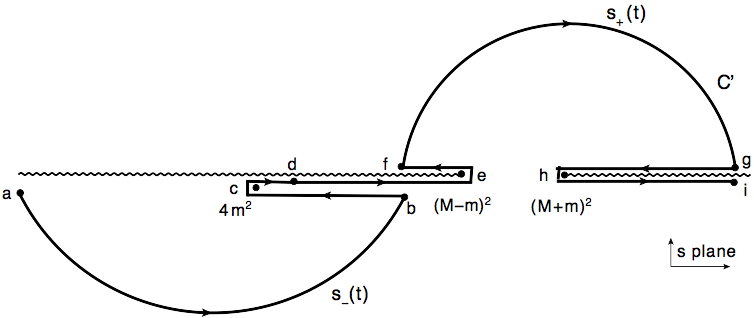
The equation for $g_{IL}$ is given by Khuri-Treiman equation, [Khuri:1960kt] [Guo:2014disp], \begin{equation} g_{IL}(s) = g_{IL}^{(0)} + \frac{1}{\pi} \int_{0}^{(M-m_{\pi})^2} dt \sum_{L'=0}^{L'_{max}}\sum_{I'} \left [ C_{st} \right]_{I I'} \big( \mathcal{K}_{IL,I;L'}(s,t) -\mathcal{K}_{IL,I'L'}(s_{0},t)\big) f_{I' L'}(t)\,g_{I'L'}(t) ,\label{gapprox} \end{equation} which is solved by matrix inversion. The subtraction constants $g_{IL}^{(0)} $ may be related to the coupling constants, and used as fitting parameters. The subtraction point is chosen to be near Adler zero, $s_{0}\simeq 4/3\,m_{\pi}^{2}$. After solving the integral equation for $g_{IL}(s)$, we compute $a_{IL}(s)$ according to Eq.(\ref{ampaIL}) and (\ref{gapprox}). The kernel function $\mathcal{K}_{IL, I' L'}(s,t)$ is given by \begin{multline} \mathcal{K}_{IL, I'L'}(s,t) = 2\,(2 L'+1) \theta(t)\,\Delta_{I L, I' L'}(s,t), \end{multline} with \begin{align} &\Delta_{IL, I'L'}(s,t) = \int_{s_{-}(t)}^{s_{+}(t)} \!\!\!\!\!\!\!\!\!\!\!\! (C') \ d s' \frac{ \rho(s')}{s'-s} \frac{(s'/4- m_{\pi}^{2})^{L}}{ \mathcal{F}_{IL}(s')\,K^{L+1}(s')/s'} \frac{ \mathcal{F}_{I'L'}(t)\,K^{L'}(t)}{(t/4- m_{\pi}^{2})^{L'}} P_{L}(z_{s'})\,P_{L'}(z_{t}) .\label{kerneldelta} \end{align} The contour ${C'}$ is given in Fig. 1.

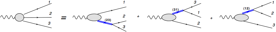
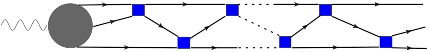
When the energy dependent amplitude $g_{IL}$ is replaced by a coupling constant, $g_{IL}^{(0)}$, the amplitudes are reduced to isobar-type model amplitudes, which we refer to two-body interaction, see Fig. 2. While the solution of Eq.(\ref{gapprox}) represent the rescattering effect among all three particles, see Fig. 3.

Dalitz distribution

It is convenient to express the amplitudes in terms of two dimensionless and independent variables $(x,y)$ which are linearly related to Mandelstam variables by the equations \begin{eqnarray}\label{defXY} x = \frac{\sqrt{3}}{2\,m_\eta\,Q_{\eta}}\,(t-u), \ \ \ \ y = \frac{3}{2\,m_\eta\,Q_{\eta}} \left ((m_\eta-m_{\pi^{0}})^{2} -s \right ) -1\,, \end{eqnarray} where $Q_{\eta} = m_\eta-2\,m_{\pi}^+-m_\pi^0$. A general property of these variables is that the physicical region of the Dalitz plot lies now inside the unit circle $x^2+y^2\leq1$ with a center at $x=y=0$.The Dalitz distribution of $\eta \rightarrow 3 \pi$ is described by \begin{align} |A^{C/N}(x,y)|^2. \end{align}

References

[WASAatCOSY:2014]
P. Adlarson et al. (WASA-at-COSY Collaboration),
``Measurement of the $\eta\rightarrow \pi^+ \pi^- \pi^0$ Dalitz plot distribution,''
Phys.Rev. C90 (2014) 4, 045207.

[GarciaMartin:2011cn]
R. Garcia-Martin, R. Kaminski, J. R. Pelaez, J. Ruiz de Elvira, and F. J. Yndurain,
``The Pion-pion scattering amplitude. IV: Improved analysis with once subtracted Roy-like equations up to 1100 MeV,''
Phys.Rev. D83 (2011) 074004.

[Khuri:1960kt]
N. N. Khuri, and S. B. Treiman,
``Pion-Pion Scattering and ${K}^{\pm}\rightarrow 3\pi$ Decay,''
Phys.Rev. 119 (1960) 1115-1121.

[Guo:2014disp]
P. Guo, I.V. Danilkin, and A. P. Szczepaniak,
``Dispersive approaches for three-particle final states interaction,''
arXiv:1409.8652.

Fitting WASA-at-COSY Dalitz Distribution

In this section, we present the fit example to Dalitz Distribution of $\eta\rightarrow \pi^+ \pi^- \pi^0$ published by WASA-at-COSY Collaboration [WASAatCOSY:2014]. Readers can choose interaction type (two-body/three-body), the number of partial waves (specified by $(I_{max},L_{max})$).

* Outputs of fitting:

Resources

The C++ code of eta to three pions decay and the instruction are available at: