We present the model published in [Nys16] .
The differential cross section for $\gamma p\to \eta p$ is computed with Regge amplitudes in the domain $E_\gamma \geq 4$ GeV and $0 \leq -t \leq 1$ (in GeV$^2$).
We use the CGLN invariant amplitudes $A_i$ defined in [Chew57a].
See the section Formalism for the definition of the variables.
The model and its context is detailed in [Nys16] . We report here only the main features of the model.

Formalism

The differential cross section is a function of 2 kinematic variables. The first is the beam energy in the laboratory frame $E_\gamma$ (in GeV) or the total energy squared $s$ (in GeV$^2$). The second is the cosine of the scattering angle in the rest frame $\cos\theta$ or the momentum transfered squared $t$ (in GeV$^2$).
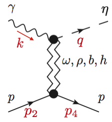
The momenta of the particles are $k$ (photon), $q$ (eta), $p_2$ (target) and $p_4$ (recoil). The eta-meson mass is $\mu$ and the proton mass is $M_N$. The Mandelstam variables, $s=(k+p_2)^2$, $t=(k-q)^2$, $u=(k-p_4)^2$ are related through $s+t+u=2M_N^2+\mu^2$. Furthermore, we introduce the crossing variable $\nu = (s-u)/(4 M_N)$.

The differential cross section ($d\sigma/{dt}$) and beam asymmetry ($\Sigma$) are expressed at leading order in $s$ in term of the invariant amplitudes $A_i$ as \begin{align}\nonumber \frac{d\sigma}{dt} = \frac{1}{32 \pi} \left( \left|A_1\right|^2 - t\left|A_4\right|^2 + \left|A_2'\right|^2 -t \left|A_3\right|^2\right) \\ \Sigma \frac{d\sigma}{dt} = \frac{1}{32 \pi} \left( \left|A_1\right|^2 - t\left|A_4\right|^2 - \left|A_2'\right|^2 +t \left|A_3\right|^2\right) \end{align} where $A_2' = A_1 + t A_2$ is introduced, since it has good quantum numbers in the $t$-channel. We will use $A_i$ as a collective notation for $(A_1, A_2', A_3, A_4)$. The differential cross section is expressed in $\mu$b/GeV$^2$. We used $(\hbar c)^2=0.3894$ mb.GeV$^2$.

The invariant amplitudes $A_i$ have good quantum numbers of the $t-$channel: the naturality $\eta=P(-1)^J$ and the product $CP$.
$C$ and $P$ are the charge conjugation and the parity. $J$ is the total spin. The amplitudes can also be decomposed into isoscalar $A_i^s$ and isovector $A_i^v$ contributions in the $t$-channel \begin{align} A_i = A_i^s + \tau_3 A_i^v \end{align} Hence, the proton and neutron amplitudes read \begin{align} A^p_i &= A_i(\gamma p \rightarrow \eta p) = A^s_i + A^v_i \\ A^n_i &= A_i(\gamma n \rightarrow \eta n) = A^s_i - A^v_i \end{align} showing that isovector contributions catch a minus sign in the neutron amplitudes.

The high-energy amplitudes are modeled by a pure Regge pole model: \begin{align} A^{\sigma}_i & = \beta^\sigma_i(t) \frac{1-e^{-i\pi\alpha_i(t)}}{\sin\pi\alpha_i(t)} (r_i\nu)^{\alpha_i(t)-1} \end{align} In Regge theory, the Regge residues are an unknown function of $t$. In order to determine the $t$-dependence, we use Finite-Energy Sum Rules (FESR) \begin{align}\label{eq:FESR_main} \frac{\pi B^\sigma_i(t)}{\Lambda} \left(\frac{\nu_M}{\Lambda}\right)^k + \int_{\nu_\pi}^\Lambda \mbox{Im} A^\sigma_i(\nu',t) \left(\frac{\nu'}{\Lambda}\right)^k \frac{d\nu'}{\Lambda} = \beta^\sigma_i(t) \frac{\left(r_i\Lambda\right)^{\alpha_i(t)-1}}{\alpha_i(t)+k} \end{align} where $\nu_\pi$ is the $\pi N$ threshold and $\Lambda$ is cut-off parameter which determines the transition between the low- and high-energy model. The first term on the LHS is due to the nucleon pole term. The second term, the dispersive integral, requires a low energy model to be integrated starting from the lowest cut. The RHS is obtained by approximating the high-energy amplitude in a Regge-pole model. By evaluating the LHS of the above FESR, one can obtain estimates on the $t$-dependence of the Regge residues $\beta_i^\sigma (t)$ of the high-energy model (RHS). In our paper [Nys16] , we use the Eta-MAID 2001 model [Chiang01] to evaluate the LHS of the sum rules. This low-energy model provides isospin decomposed amplitudes and is valid up to $\sqrt{s} = 2.0 \mbox{ GeV}$.

Model

The model is based on the exchange of the leading Regge singularities.
We show here only the 'conservative model' in [Nys16] . Since $C\ket{\gamma\eta} = -\ket{\gamma\eta}$, the only quantum numbers allowed in the $t-$channel are \begin{align} \rho &: I^{G\tau\eta}=1^{+-+}, & A_1,A_4\\ \omega &: I^{G\tau\eta}=0^{--+}, & A_1,A_4\\ b &: I^{G\tau\eta}=1^{+--}, & A_2\\ h &: I^{G\tau\eta}=0^{---}, & A_2\\ \rho_2 &: I^{G\tau\eta}=1^{++-}, & A_3\\ \omega_2 &: I^{G\tau\eta}=0^{-+-}, & A_3\\ \end{align} The second column indicates the amplitudes which the exchange contributes to.
$G=C(-1)^I$ is the $G-$parity and $\tau=(-1)^J$ is the signature.
The quantum numbers of the trajectories are denoted by the lowest spin particles.
We will refer to vector for the $\rho$ and $\omega$ trajectories and to axial-vector for the $b$ and $h$ trajectories. The $A_1$ ($A_4$) amplitude is related to an $s$-channel nucleon-helicity flip (non-flip) contribution. The $A_3$ has quantum numbers which do not correspond to any observed meson. We therefore do not include $A_3$ contributions in our model.

The $t$ dependence of the amplitudes is estimated by matching the exchange of the lowest particles in the CGLN basis. The amplitudes involve the vector ($\alpha_V$) and axial-vector ($\alpha_A$) poles \begin{align} A_1 &= g_1^V t R(\alpha_V) ,& A_2'&= g_2^A t R(\alpha_A),& A_3&=0,& A_4 &= g_4^V R(\alpha_V). \end{align} The $g_i$ are real fitting parameters, corresponding to the coupling constants.
The $s$-dependence of the high-energy amplitude is given by the Regge prescription. For the $t$-dependence, we use the above estimate, in combination with features that are present in the LHS prediction of the FESR. From matching with the LHS of the sum rules, we assume the following paramerization for a given isospin component $\sigma = s,v$ \begin{align} A_1^\sigma &= g_1^V t \frac{ -\pi \alpha_V' }{\Gamma(\alpha_V + 1)} \frac{1 - e^{-i\pi\alpha_V}}{2 \sin \pi \alpha_V} \left(r_1 s\right)^{\alpha_V - 1} \label{eq:A1},\\ A_2^{\prime \sigma} &= g_2^A t \frac{ -\pi \alpha_A' }{\Gamma(\alpha_A + 1)} \frac{1 - e^{-i\pi\alpha_A}}{2 \sin \pi \alpha_A} \left(r_2 s\right)^{\alpha_A - 1} ,\\ A_3^\sigma &= 0,\\ A_4^\sigma &= g_4^V \frac{ -\pi \alpha_V' }{\Gamma(\alpha_V)} \frac{1 - e^{-i\pi\alpha_V}}{2 \sin \pi \alpha_V} \left(r_4 s\right)^{\alpha_V - 1} \label{eq:A4}, \end{align} where for $\sigma = s$ ($\sigma = v$) we have $V = \omega$ and $A = h$ ($V = \rho$ and $A = b$). We introduced the scaling parameters $r_{i=1,2,4}$, which are fitted to the data. Finally we use linear Regge trajectories \begin{align} \alpha_V(t) &= \alpha_{V0}+ \alpha_V' t = 1 + 0.9(t - m_\rho^2),\\ \alpha_A(t) &= \alpha_{A0}+ \alpha_A' t = 0 + 0.7(t - m_\pi^2). \end{align}

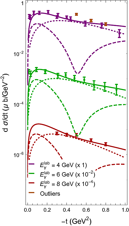
We have fitted 8 parameters to the available data. The result is \begin{align} \label{eq:param1} g_1^\rho &= \phantom{+} 3.434 \pm 0.083 \mbox{ GeV}^{-2}, & g_2^b &= \phantom{+} 4.946 \pm 1.491 \mbox{ GeV}^{-2}, & g_4^\rho &= -1.397 \pm 0.085 \mbox{ GeV}^{-1},\\ g_1^\omega &= \phantom{+} 0.116 \pm 0.074 \mbox{ GeV}^{-2},& g^h_2 & = (2/3) g^b_2, & g_4^\omega &= -3.346 \pm 0.087 \mbox{ GeV}^{-1},\\ r_1 &= \phantom{+}3.001 \pm 0.087 \mbox{ GeV}^{-1}, & r_2 &= \phantom{+}6.204 \pm 2.484 \mbox{ GeV}^{-1}, & r_4 &= \phantom{+}1.974 \pm 0.101 \mbox{ GeV}^{-1}. \end{align}

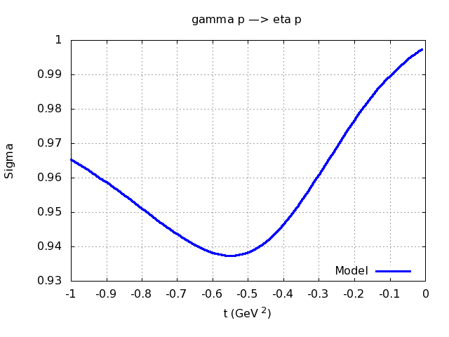
The results is presented below and compared to the data from [Dewire71] and [Braunschweig70]. The dashed (dotted-dashed) line indicates the isoscalar (isovector) contribution. One clearly observes that the dominant $s$-channel helicity flip component of the $\rho$ dominates the cross section (except at very forward angles). Since it lacks a nonsense-wrong-singature zero, it does not introduce a dip in the cross section. This mechanism uses a natural-parity exchange term to fill up the dip that is expected from the similar $\pi^0$ photoproduction reaction. By measuring the photon beam asymmetry at high energies, one can verify whether the dip-filling mechanism should indeed be attributed to natural exchanges. A measurement of the beam asymmetry $\Sigma$ close to $+1$ would support the dominance of natural exchange and our model. Our model prediction for the beam asymmetry, presented below at $E_\gamma=9$ GeV, is indeed close to 1.

References

[Nys16]
J. Nys et al.,
``Finite-Energy Sum Rules in Eta Photoproduction of the Nucleon,'' Phys. Rev. D 95, 034014 (2017)

[Chiang01]
W. T. Chiang et al.,
``An Isobar model for eta photoproduction and electroproduction on the nucleon,'' Nucl. Phys. A700, (2002) 429.

[Chew57a]
G.F. Chew, M.L. Goldberger, F.E. Low and Y. Nambu,
``Relativistic dispersion relation approach to photomeson production,'' Phys. Rev. 106, (1957) 1345.

[Dewire71]
J. Dewire et al.,
``Photoproduction of eta mesons from hydrogen," Phys. Lett. B37 (1971) 326.

[Braunschweig70]
W. Braunschweig et al.,
``Single photoproduction of eta-mesons on hydrogen in the forward direction at 4 and 6 Gev," Phys. Lett. B33 (1970) 236.

Resources

Below we provide a number of C/C++ codes to evaluate the model. A first code ("C/C++ observables") is the code which is used to calculate the observables on this webpage. It includes a rotation of the invariant amplitudes $A_i$ basis to the helicity amplitudes $H_i$, in order to evaluate the observables with their exact expressions. This code evaluates the Eta-MAID 2001 model when $W \leq 2 \mbox{ GeV}$. A second and lighter code ("C/C++ minimal code to calculate the amplitudes") contains the minimal amount of code to evaluate the invariant amplitudes $A_i$ of the high-energy Regge model. This does not include the Eta-MAID 2001 model. Below we describe in detail how to use the latter code. We suggest using the minimal script to calculate any observable. This avoids mixing various conventions for the polarization observables and/or misinterpretations of the code. As a check, one can reconstruct the beam asymmetry and differential cross section provided in the interactive part below (see section "Run the code").

• Publication: [Nys16]
• C/C++ observables: C-code main, Input file, C-code source, C-code header, Eta-MAID 2001 multipoles
• C/C++ minimal script to calculate the amplitudes: C-code zip
• Data: Dewire , Braunschweig
• Contact person: Jannes Nys, Vincent Mathieu
• Last update: November 2016

Run the code